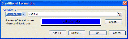
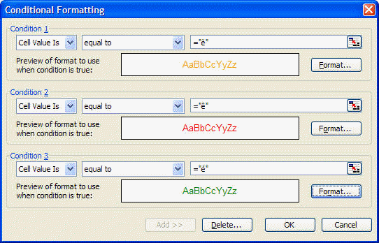
Mimic 2007 Conditional Formatting Icons

XL2007 has a extended conditional formatting to allow the display of icon sets. The following will demonstrate some ways in which you can create a similar appearance in previous versions of excel.

Here is how XL2007 would display a small data table. The shift arrows are based on the difference between 2007 and 2006 Performance figures for each Widget.

The 4 Rating columns are based on the comparison of the Sales of the Widgets. Here is the same data table in xl2003 The arrows are the easiest to construct as this are based on characters from the Wingdings font.
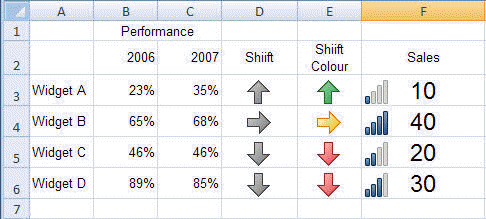
The cell D3 contains the following formula
Lets break that formula down. The MID function returns a sub set of characters from a piece of text starting at a specific position and continuing for a specified number of characters. The piece of text is "èéê" which displayed using the wingdings font is èéê. The number of character we want displayed is always 1. The start position is determined by the compound IF function. The first test is for the 2 values being equal. If they are the number 1 if returned and used as the starting position. If not the second IF function is performed. If the difference between the 2007 and 2006 value is positive 2 is returned otherwise 3.
The Shift Colour column contains the same formula in order to get the correct arrow displayed. The colour is provided by using normal conditional formatting. The ratings icon requires some additional work to create the picture we will need in order to mask conditional formatting of cells.
Start by creating 4 rectangular auto shapes increasing in size. Position these in front of a larger white rectangle with no border.
Note: For the purposes of this page I have coloured the background shape so you can see it against a white background.
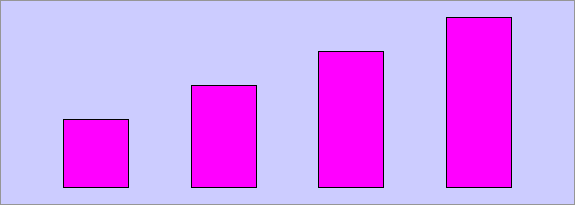
Select all five shapes and group them. Now whilst holding the SHIFT key click the Edit menu. You should see a new menu item Copy Picture... You will then see a dialog that allows you copy the shape as a BMP picture. Once you have copied the picture use paste to insert the new picture back into your workbook. If you select the picture you should see the Picture toolbar, if not right click the picture and pick Show Picture Toolbar... 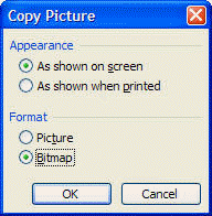You can now use the Set Transparent Color button to turn those Pink bars see-thru. Size and position the picture over the range G3:J3. The 4 columns are going to provide the colour for the bars but in order to get the correct number display we need a calculate how many to display and then apply conditional formatting on each column.
Lets start with the formula to calculate whether to display 1, 2, 3 or 4 bars. Note that with the 4 rating bar 1 is always displayed so we can already set the fill colour of the cells in column G to Blue.
This is the formula in G3
It calculates the percent value of the spread of a Sales figure in relations to all the Sales figures (I think!). The percentage is then used as the lookup value in the table with the following outcome
4 bars when value is >= 75%
3 bars when value is >=50% AND < 75%
2 bars when value is >=25% AND < 50%
1 bar when value is  <25%

Now we need to apply conditional formatting to H3:H6 The conditional formatting for columns I and J is the same except the >1 part change to >2 and >3 respectively. You should now have cells displaying a blue pattern depending on the number in column G. The picture acts as a mask over those 4 columns. Here is the example workbook CF_Icons_2003