| |
| |
|
| |
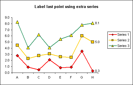
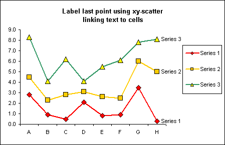
Step by step instructions for
creating a chart that displays a value label on the last point.
Based on the data below.
|
|
A
|
B
|
C
|
D
|
E
|
F
|
G
|
1
|
|
Series 1
|
Series 2
|
Series 3
|
Label Last 1
|
Label Last 2
|
Label Last 3
|
2
|
A
|
2.8
|
4.5
|
8.3
|
=IF($A3="",B2,NA())
|
=IF($A3="",C2,NA())
|
=IF($A3="",D2,NA())
|
3
|
B
|
0.9
|
2.3
|
4.1
|
=IF($A4="",B3,NA())
|
=IF($A4="",C3,NA())
|
=IF($A4="",D3,NA())
|
4
|
C
|
0.5
|
2.8
|
6.2
|
=IF($A5="",B4,NA())
|
=IF($A5="",C4,NA())
|
=IF($A5="",D4,NA())
|
5
|
D
|
2.1
|
3.1
|
4.1
|
=IF($A6="",B5,NA())
|
=IF($A6="",C5,NA())
|
=IF($A6="",D5,NA())
|
6
|
E
|
0.8
|
2.6
|
5.5
|
=IF($A7="",B6,NA())
|
=IF($A7="",C6,NA())
|
=IF($A7="",D6,NA())
|
7
|
F
|
0.9
|
2.5
|
6.1
|
=IF($A8="",B7,NA())
|
=IF($A8="",C7,NA())
|
=IF($A8="",D7,NA())
|
8
|
G
|
3.5
|
6
|
7.8
|
=IF($A9="",B8,NA())
|
=IF($A9="",C8,NA())
|
=IF($A9="",D8,NA())
|
9
|
H
|
0.3
|
5
|
8.1
|
=IF($A10="",B9,NA())
|
=IF($A10="",C9,NA())
|
=IF($A10="",D9,NA())
|
10
|
|
|
|
|
|
|
|
Use the chart wizard to create a line
chart based on A1:G9
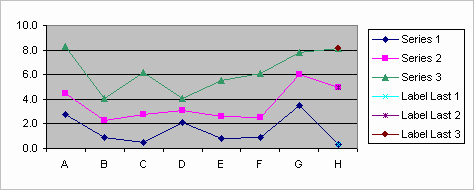
Select the 4th data series 'Label
Last 1' and format series to have border and marker None. Also enabled
Data Label Value. Repeat for 5th and 6th data series.
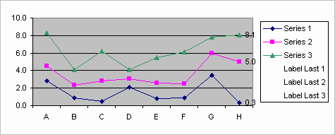
Format the plot area as required.
Here I have removed the border, major gridlines and changed the plotarea
colour.
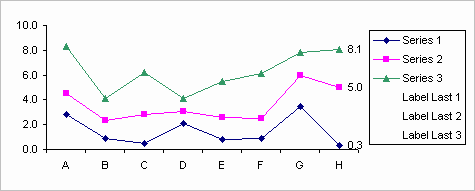
Finally remove the additional data
series from the legend.
Select the legend and then select the data series. Make sure the
selection include both marker and text otherwise the data will be
deleted.
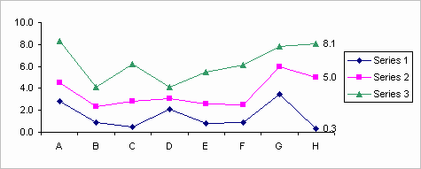
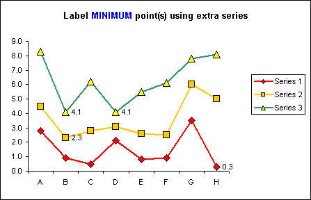
Here are some other examples of
alternative methods and application.
The workbook
contains step by step explanations on how to construct the charts using
all of the different methods.
|
|
|
|

 AJP Excel Information